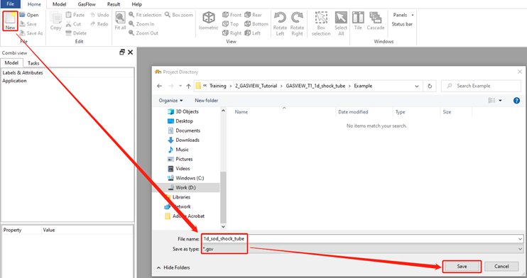
Step 1. Create a New Project
After opening GASVIEW, create a new project file named 1d-sod-shock-tube.gsv.
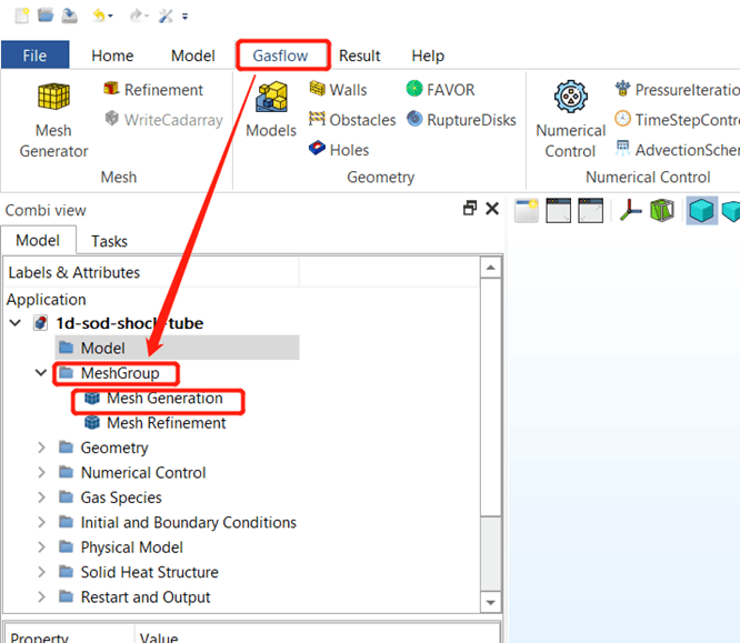
Step 2. Generate Mesh
There is no need to build a CAD model since it is a 1D problem.
Note: the default Unit system in GASFLOW is cm-g-s.
2.1 Click Gasflow - MeshGroup - Mesh Generation
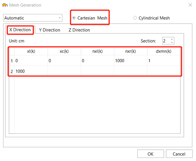
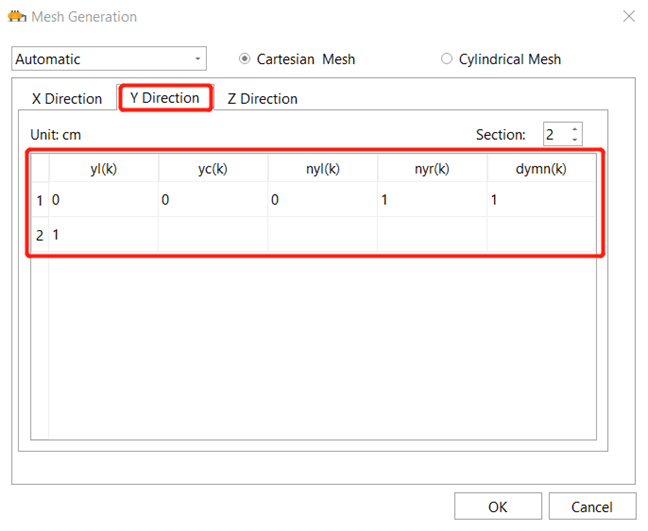
2.2 Generate mesh in Cartesian coordinate using the simple mesh generator in GASFLOW: 1000 cells in X Direction, 1 cell in Y Direction and 1 cell in Z Direction.
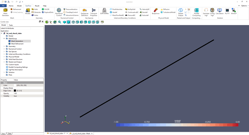
Step 3. Create the Geometry Model
3.1 a 1D tube with 1000 cells is created.
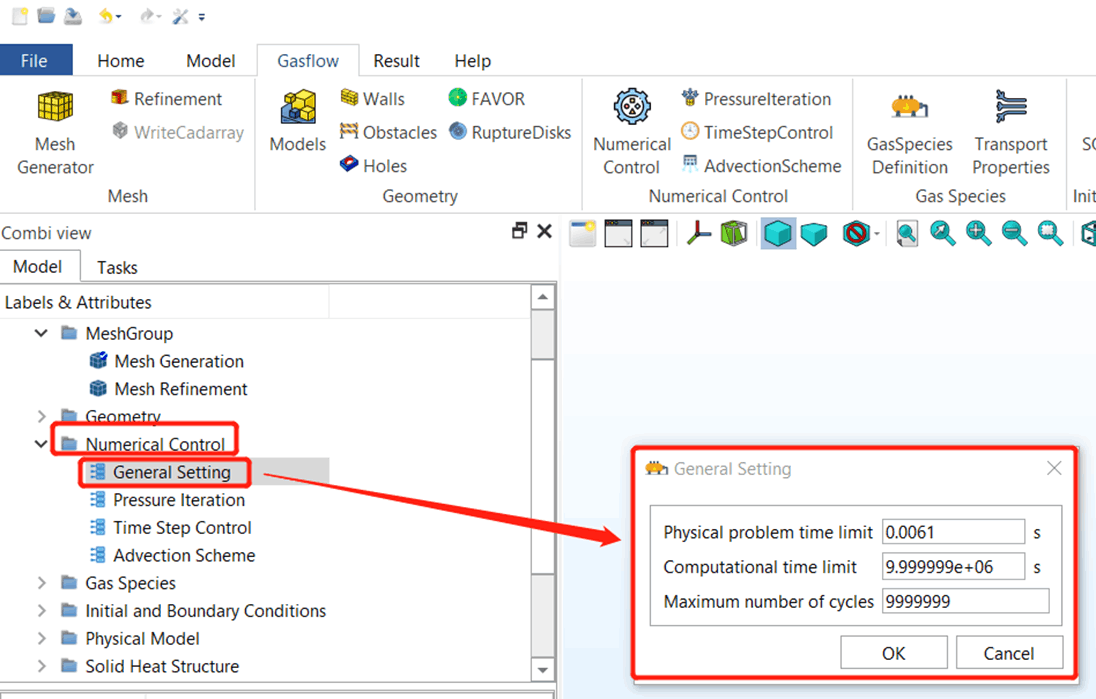
Step 4. Numerical Setup
4.1 Set up the physical and computational time. The GASFLOW results will be compared to the analytical solutions at 0.0061 s.
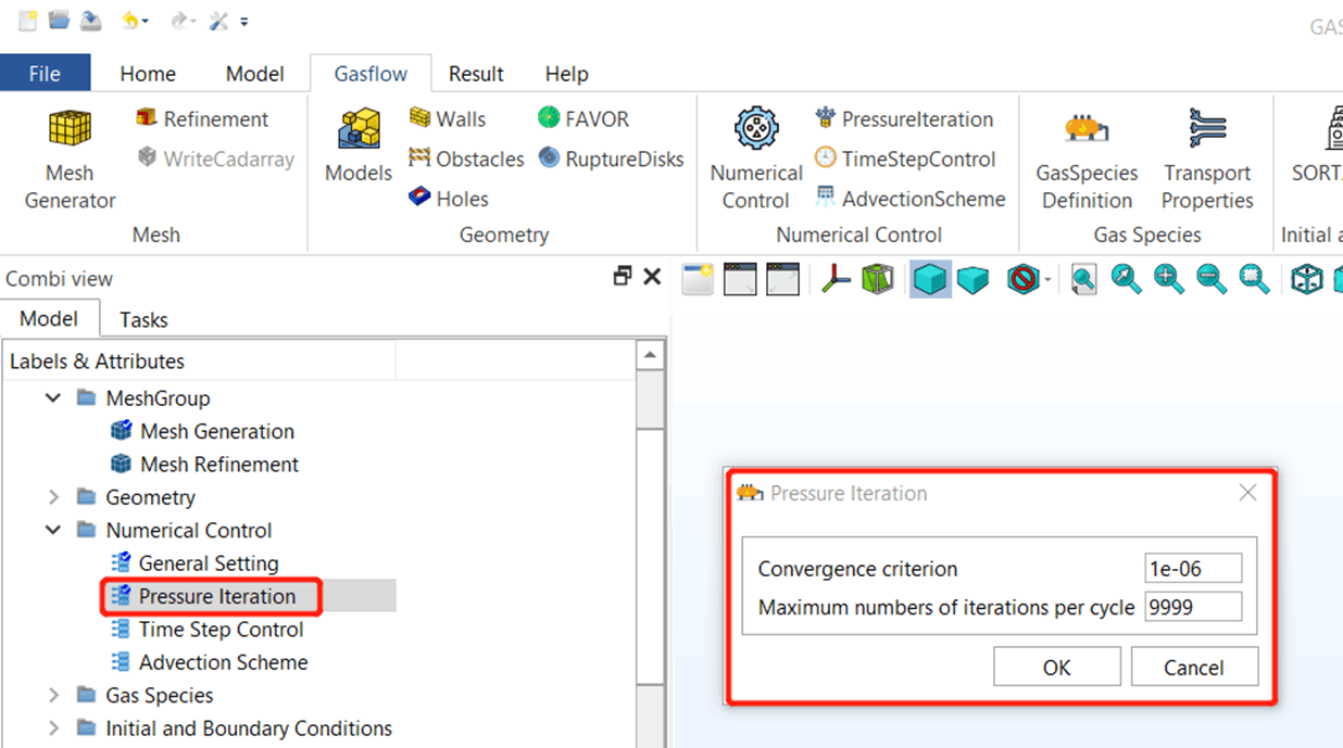
4.2 Set up the convergence criterion for pressure iteration
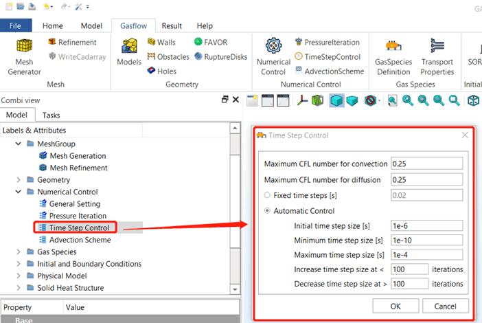
4.3 Time step control
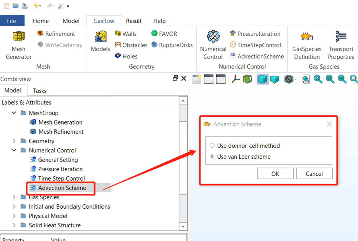
4.4 Set up the numerical scheme
5. Gas Species and Thermophysical Properties
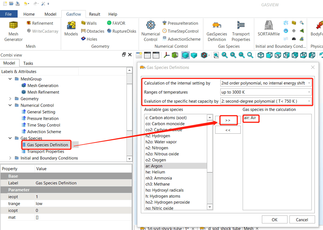
5.1 Select gas species and define the options for thermophysical properties
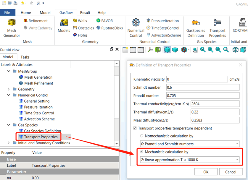
5.2 Define the options for transport properties
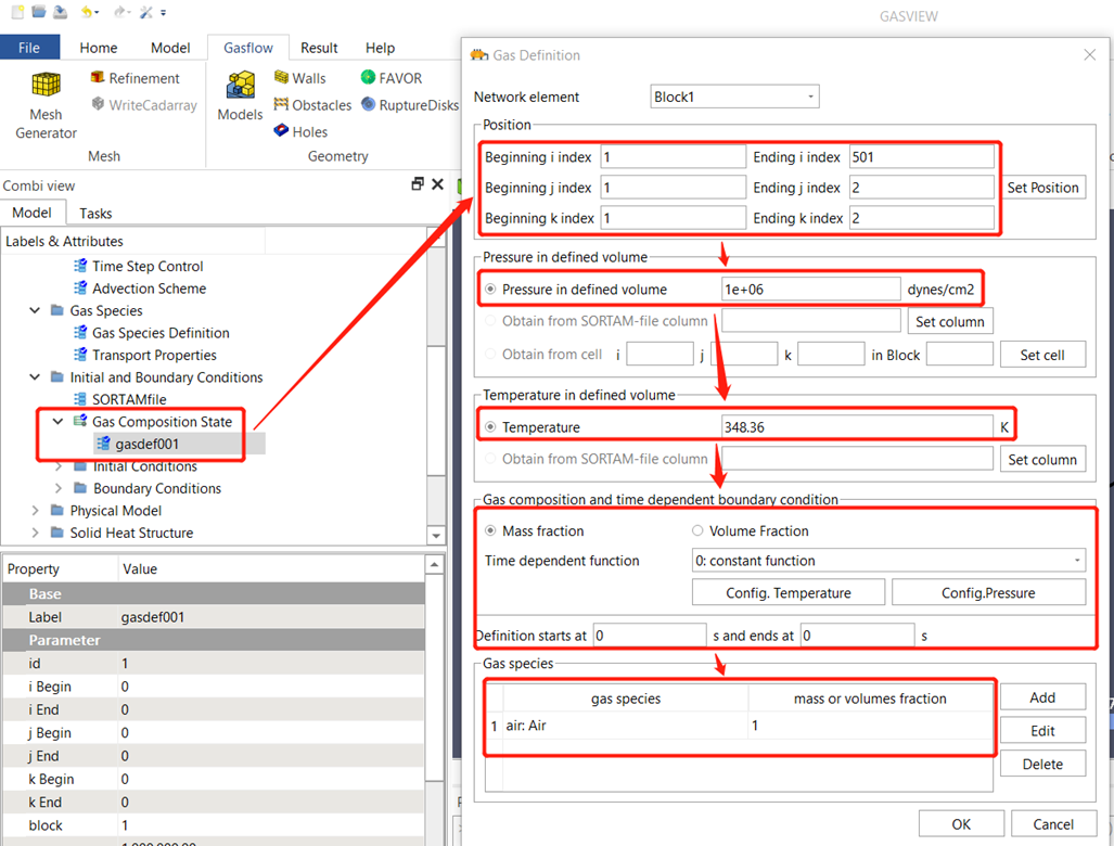
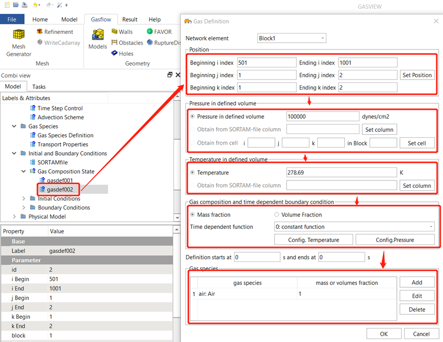
Step 6. Initial Conditions
6.1 Set up the initial condition in the higher pressure part
6.2 Set up the initial condition in the lower pressure part
6.3 Set up the initial velocity (0 cm/s) in the tube.

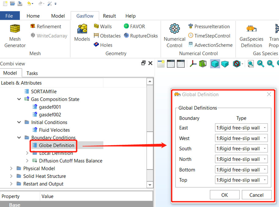
Step 7. Boundary Conditions
7.1 Set up boundaries.
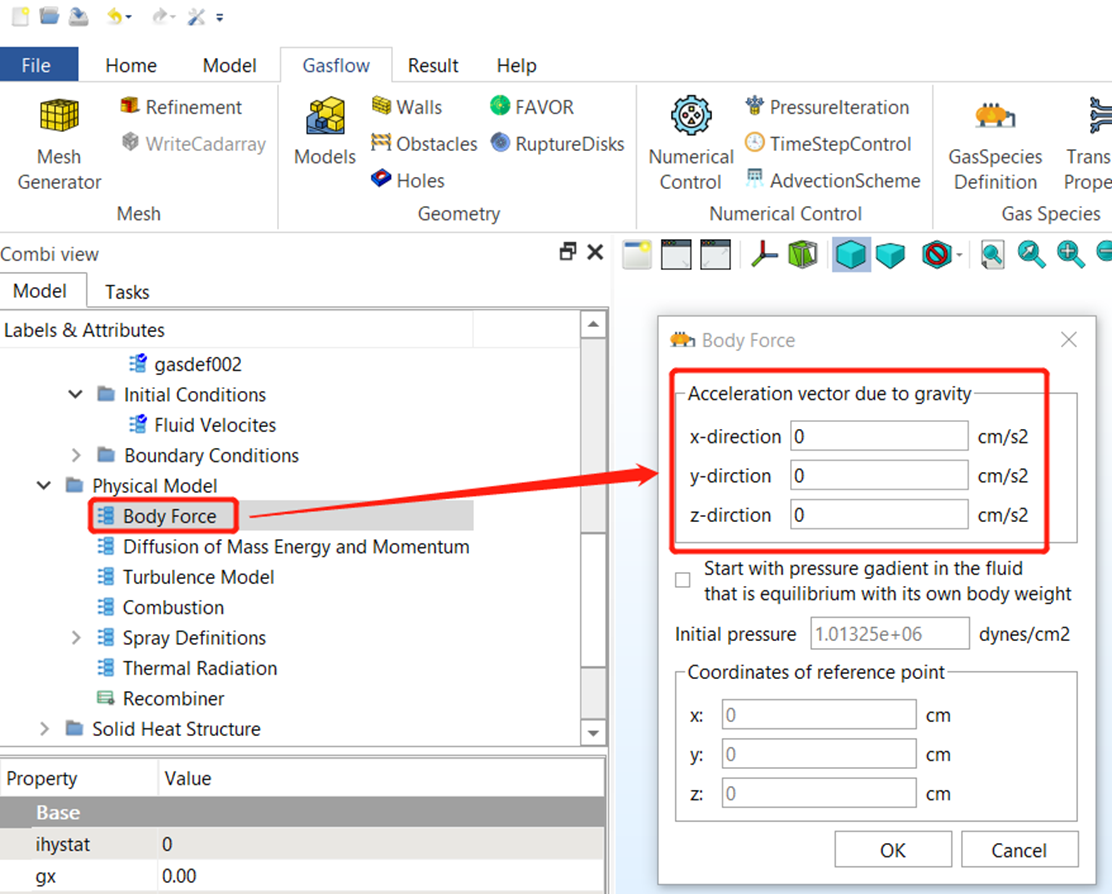
Step 8. Physical Models
8.1 Physical model setup is not required since the Euler equation is solved in this problem. The user could deactivate the gravitational force which of course has no effect on the results.
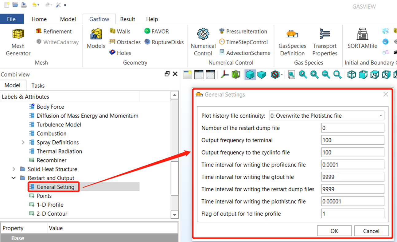
Step 9. Restart and Outputs
9.1 General options.
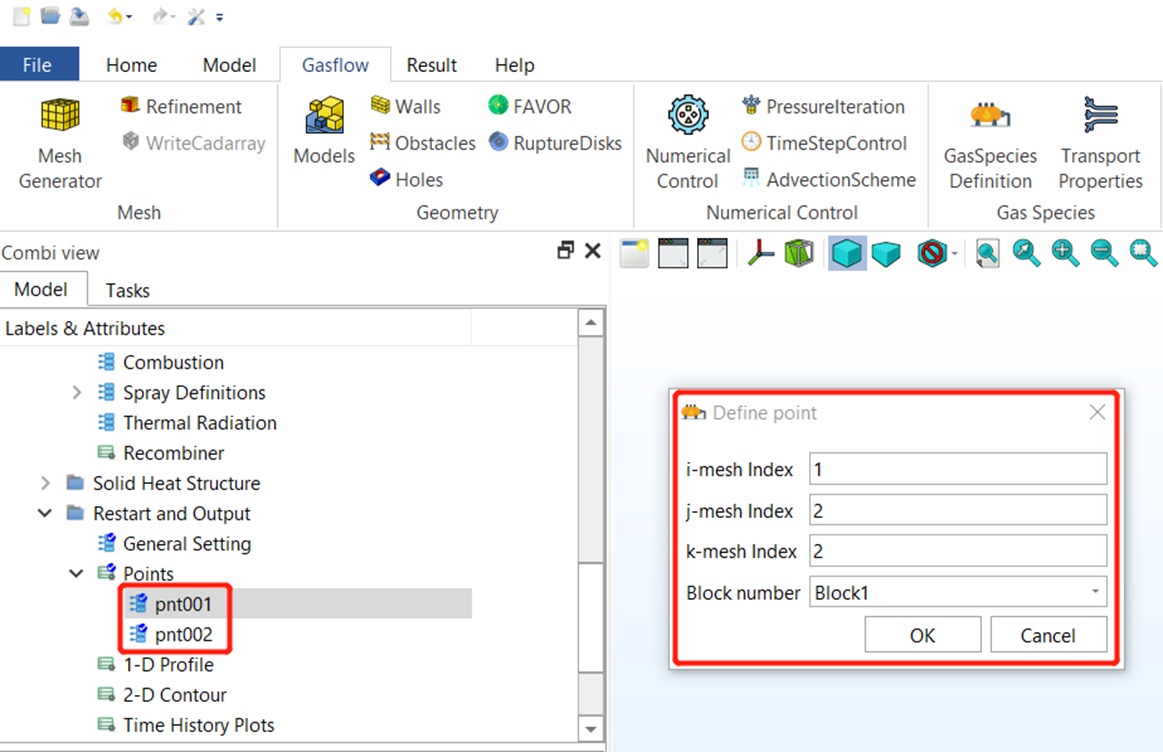
9.2 Define two points: pnt001 (i=1, j=2, k=2) and pnt002 (i=1001, j=2, k=2).
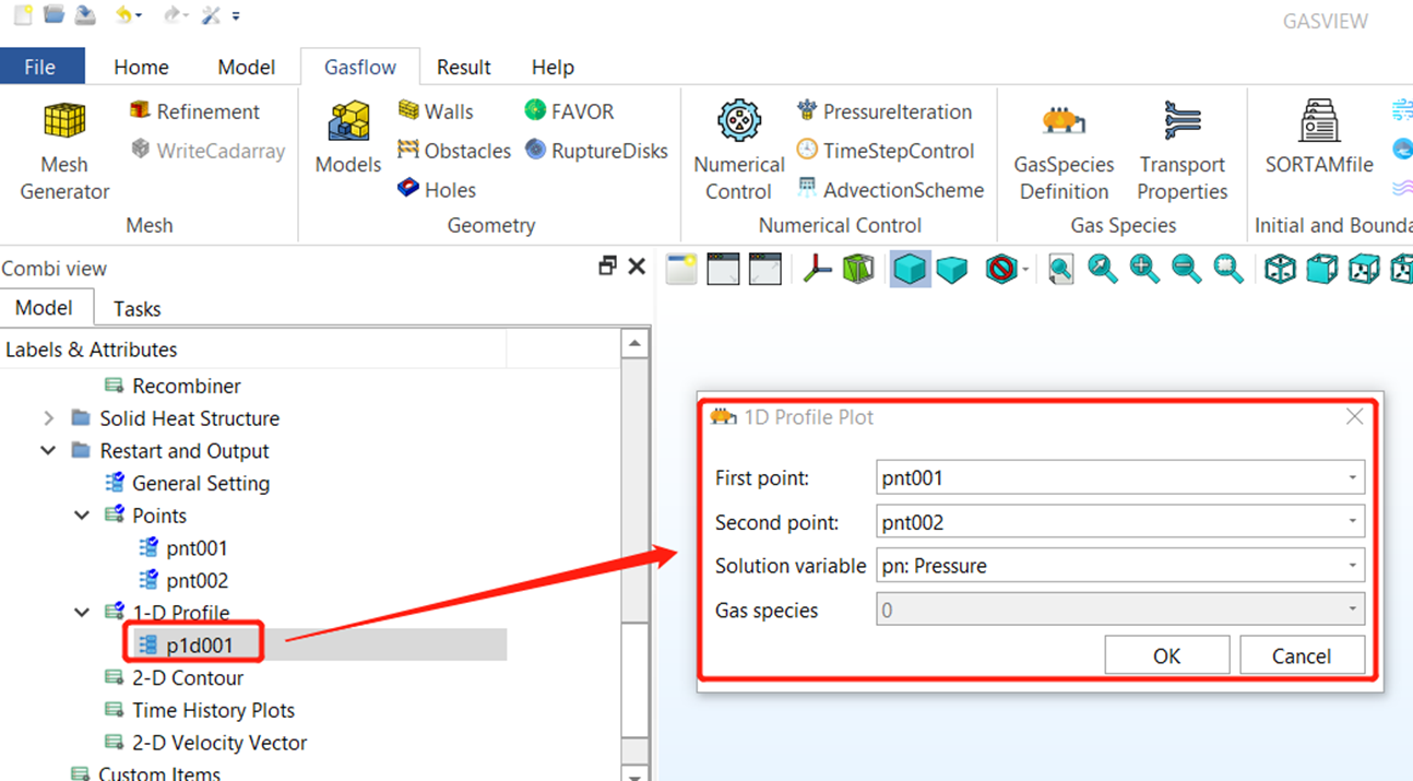
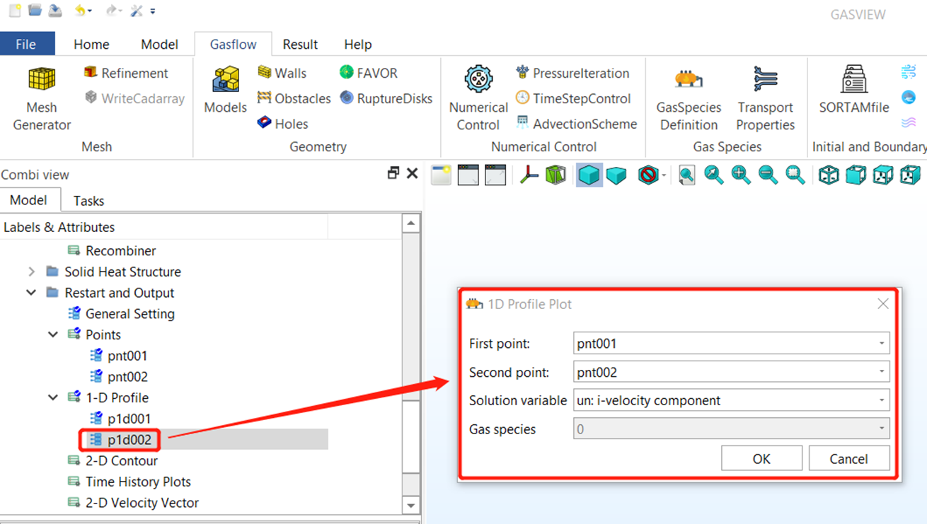
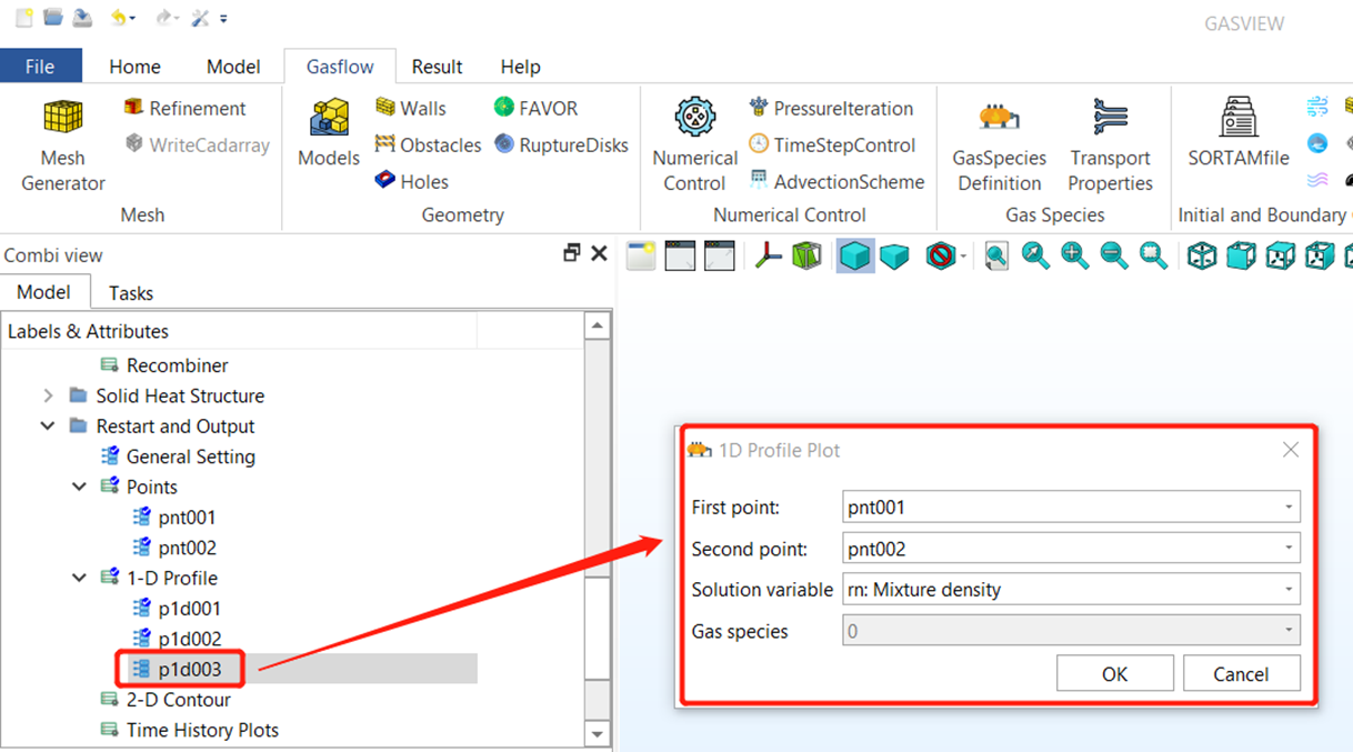
9.3 Define 1D profiles along the tube for plotting the variable "Pressure", "i-velocity component" and "Mixture Density".
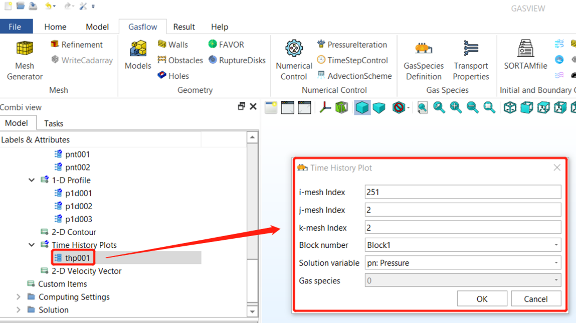
9.4 Define a monitor point (i = 251, j = 2, k = 2) to plot the time history of the variable "Pressure".
Step 10. Generate Input File
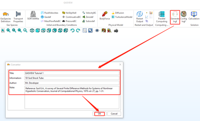
10.1 Click "Generate Ingf". Input information and click "OK" to automatically generate the input file.
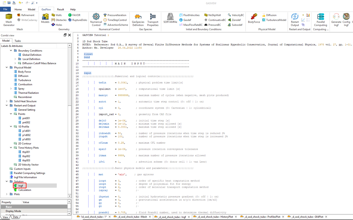
10.2 Click "Ingf" to review the input options. (ingf file)
Step 11. Run Simulation
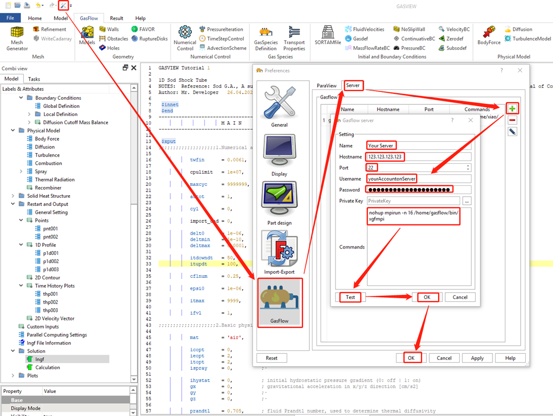
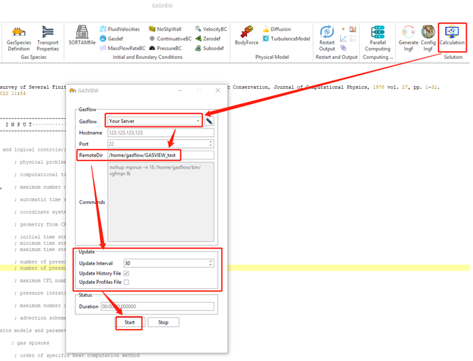
11.1 Set up the GASFLOW server.
11.2 Click "Calculation", set up the running directory and run GASFLOW.
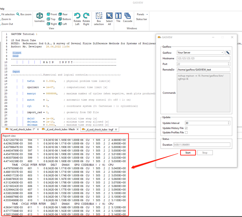
11.3 The calculation cycle information is shown in the "Report View".
Step 12. Post-processing
12.1 Click "Plots" - "HistoryPlot" to draw the time history plots.
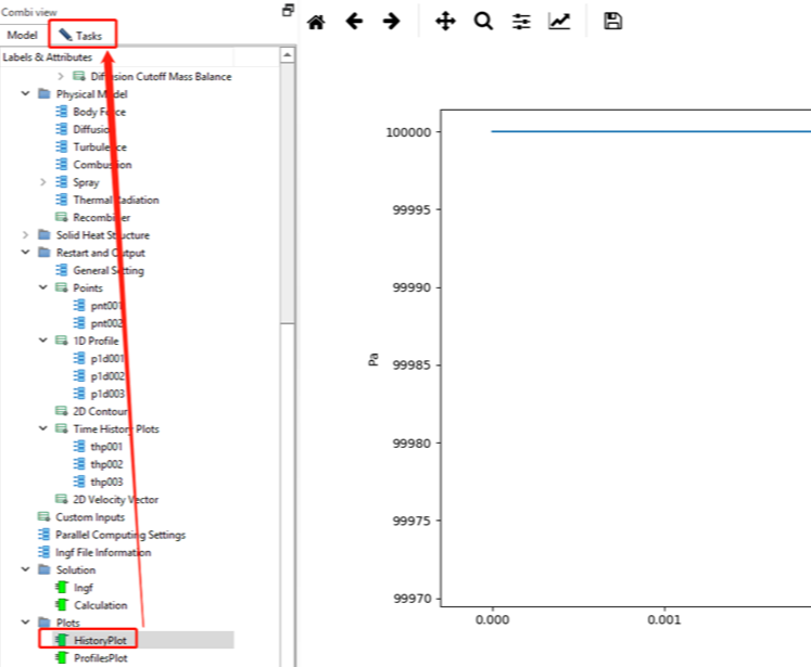
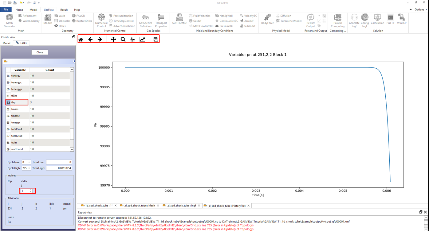
12.2 Click "thp" to plot time history of the variables defined in Step 9.
12.3 Click "ProfilesPlot" to plot 1D profiles of the variables defined in Step 9.

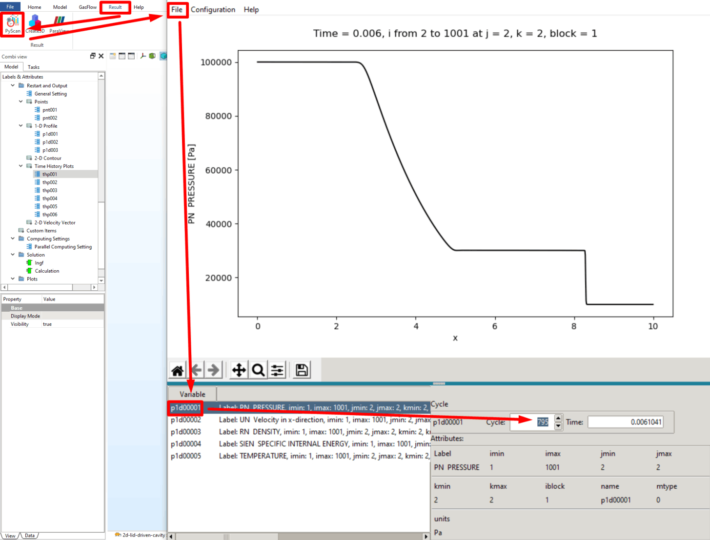
12.4 The user can also open "pyscan" in "Results - PyScan" to read the "plothist.nc" and "profiles.nc" files in the "output" directory. More details of using pyscan can be found in https://docs.gasflow-mpi.com/4.-tools/4.1.-pyscan
Files for 1D shock tube tutorial
GASVIEW project file, GASFLOW input file and GASFLOW results files can be downloaded in the link:
https://docs.gasflow-mpi.com/2.-tutorials/2.2.-running-first-tutorial/2.1.13.-downloads