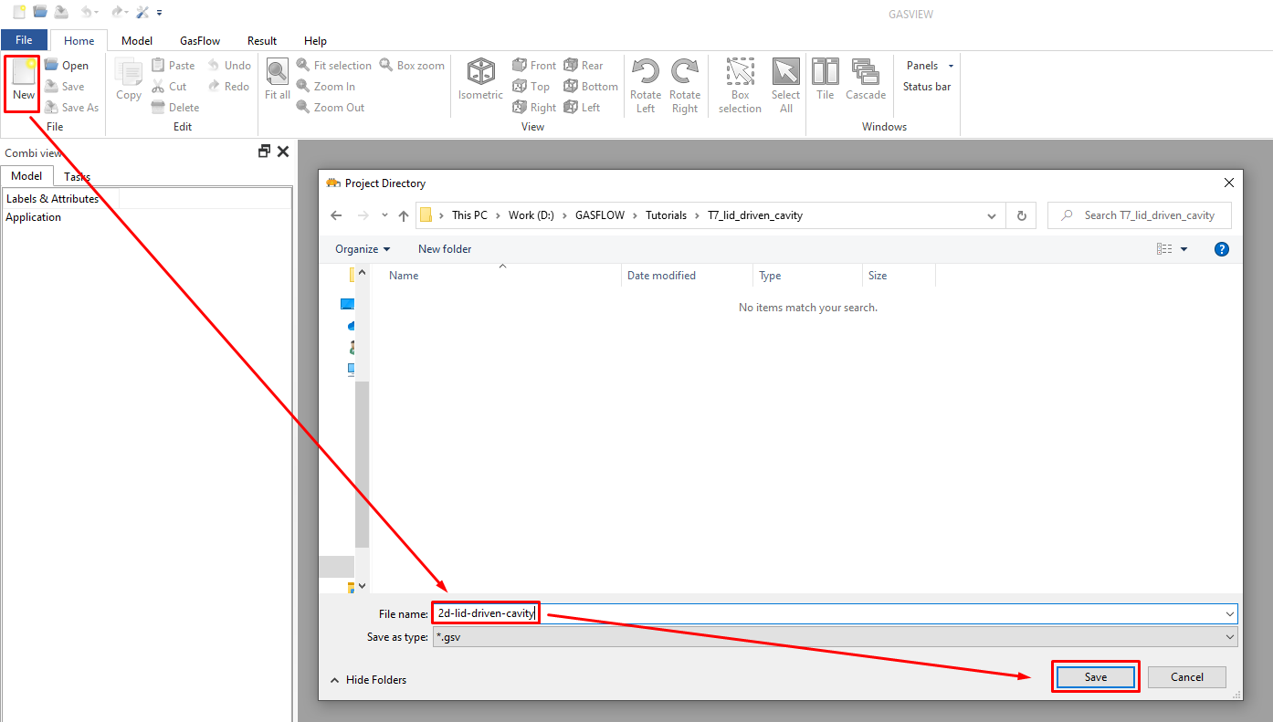
Step 1. Create a New Project
After opening GASVIEW, create a new project file named 2d-lid-driven-cavity.gsv.
Step 2. Generate Mesh
There is no need to build a CAD model since it is a simple problem with 2D geometry.
Note: the default Unit system in GASFLOW is cm-g-s.
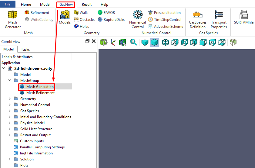
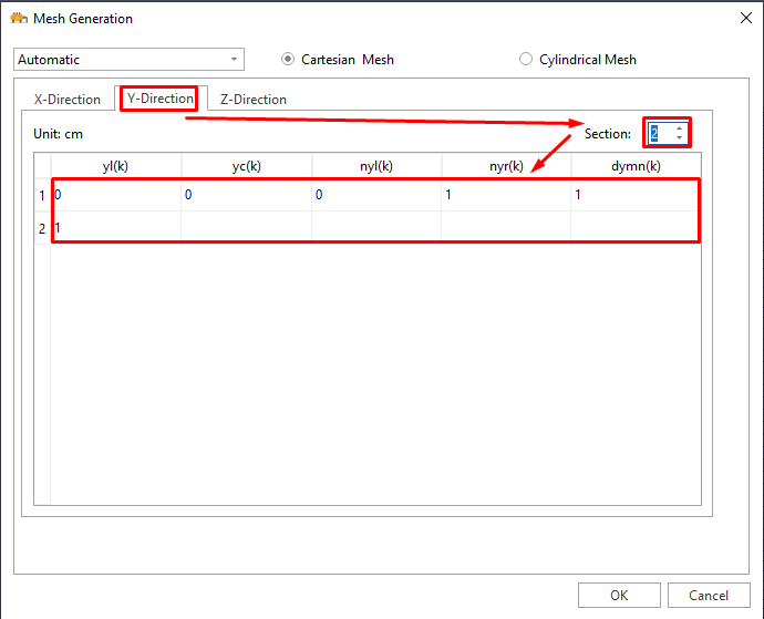
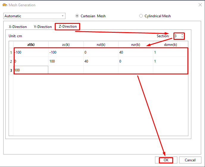
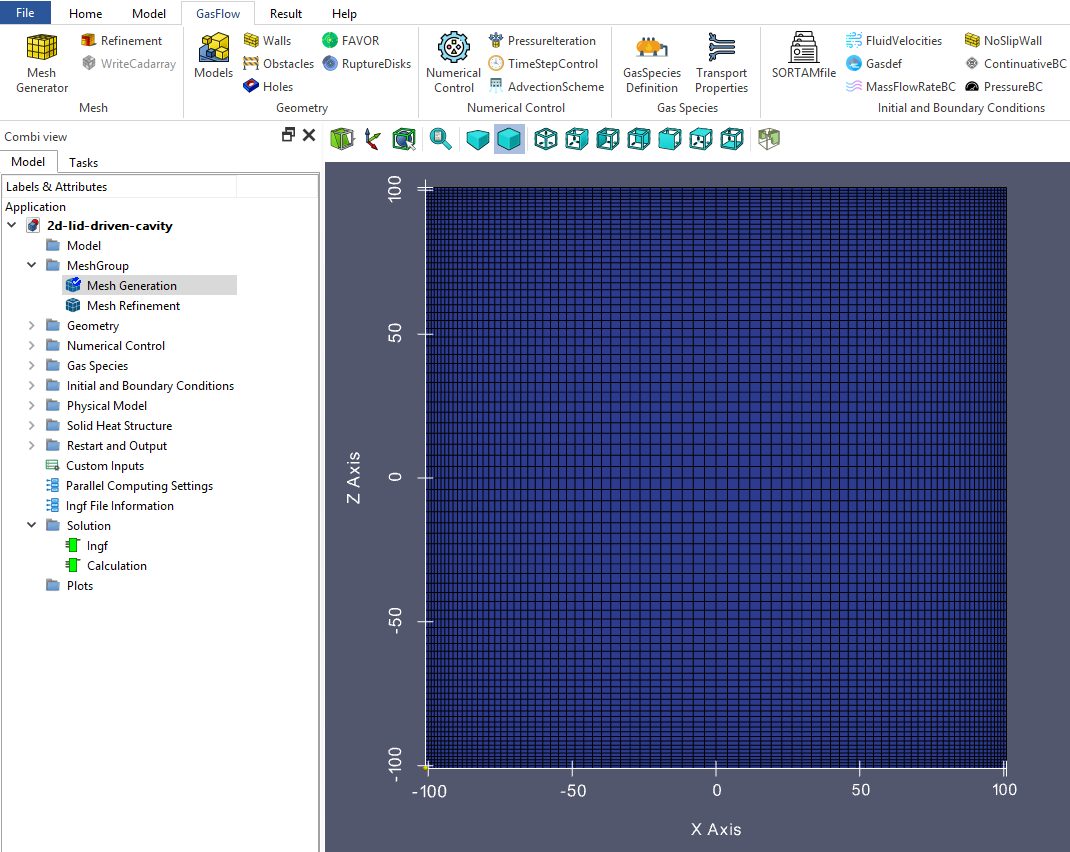
2.1 Click Gasflow - MeshGroup - Mesh Generation
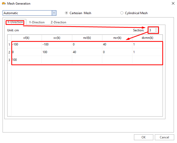
2.2 Generate mesh in Cartesian coordinate using the simple mesh generator in GASFLOW: 80 cells in X Direction, 1 cell in Y Direction and 80 cells in Z Direction. The minimum cell size near the wall is 1 cm.
Step 3. Create the Geometry Model
3.1 a 2D plane (X-Z) with 40*40 cells is created.
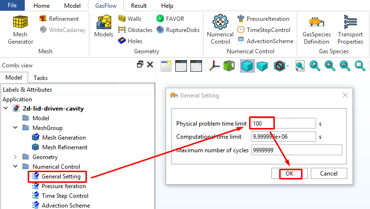
Step 4. Numerical Setup
4.1 Set up the physical time to 100 s which should be sufficiently long to reach the steady state. Use the default values for the computational time limit (9.999999e+06) and maximum number of cycles (9999999).
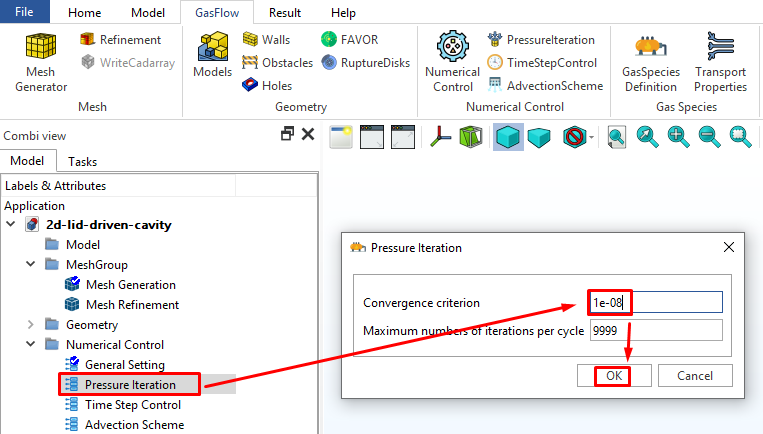
4.2 Set up the convergence criterion for pressure iteration (1e-8).
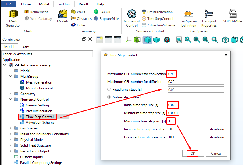
4.3 Time step control. Set the "Maximum CFL number for convection" to 0.9 to allow a larger time step. Set the "Initial time step size" to 0.02 s which is between the "Minimum time step" (1e-4 s) and the "Maximum time step" (1.0 s).
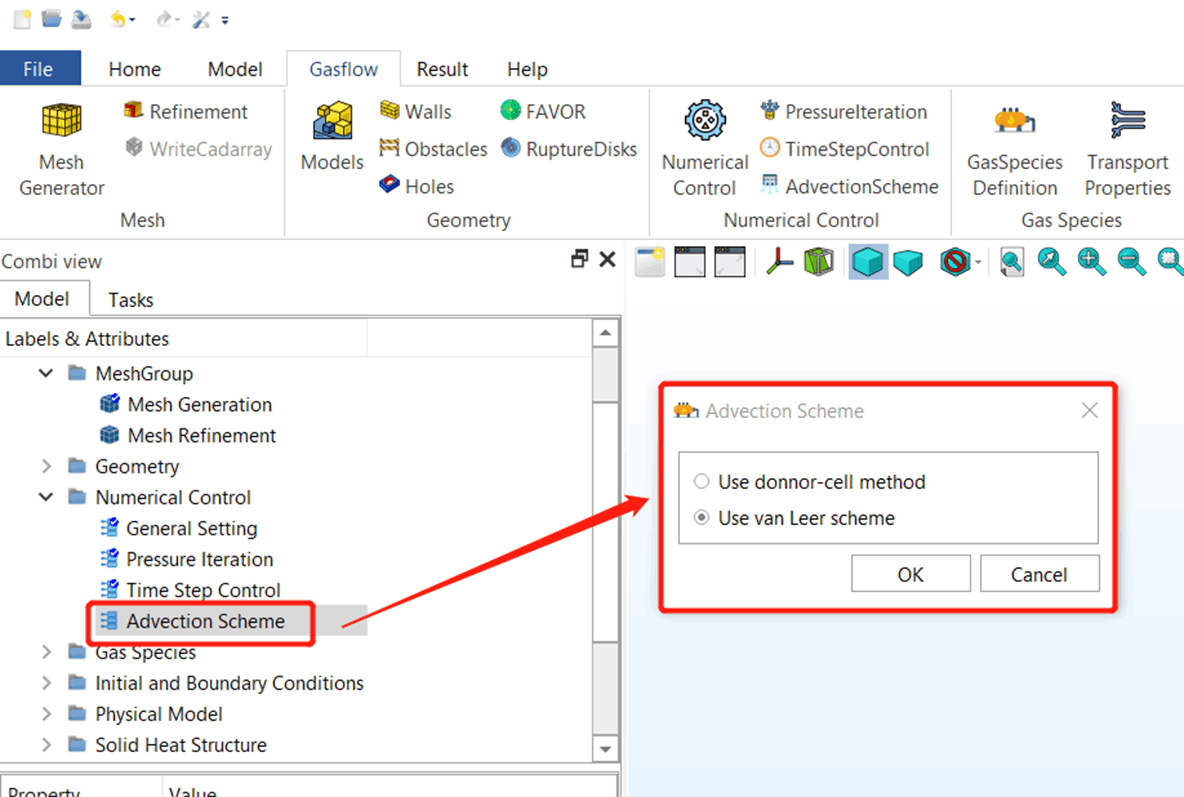
4.4 Set up the numerical scheme: second order Van Leer scheme
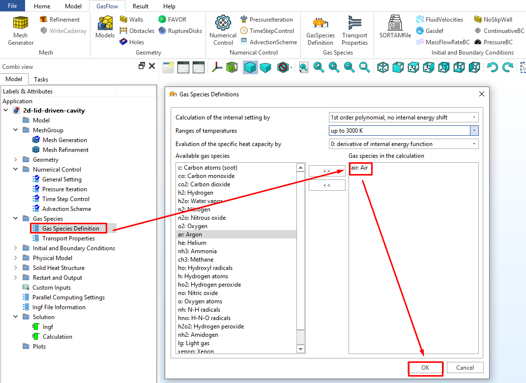
5. Gas Species and Thermophysical Properties
5.1 Select gas species and define the options for thermophysical properties
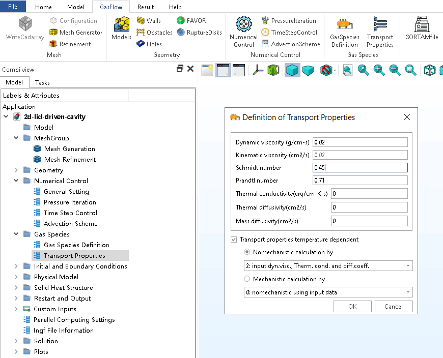
5.2 Define the options for transport properties
Step 6. Initial Conditions
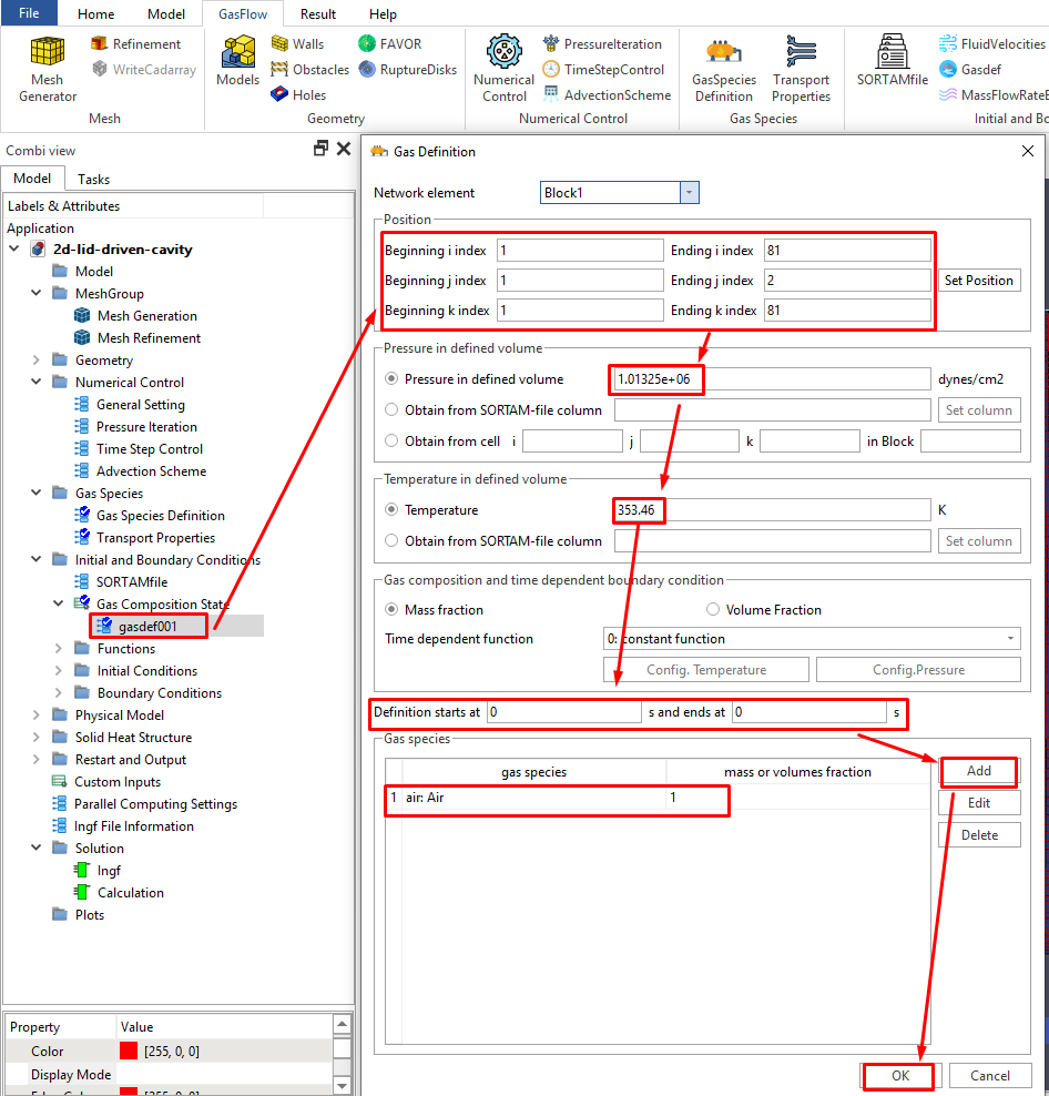
6.1 Set up the initial condition in the cavity.
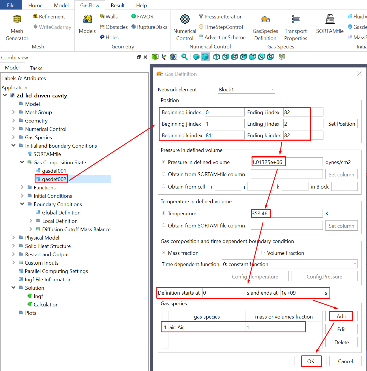
6.2 Set up the constant condition in the ghost cells where the lid is located.
Step 7. Boundary Conditions
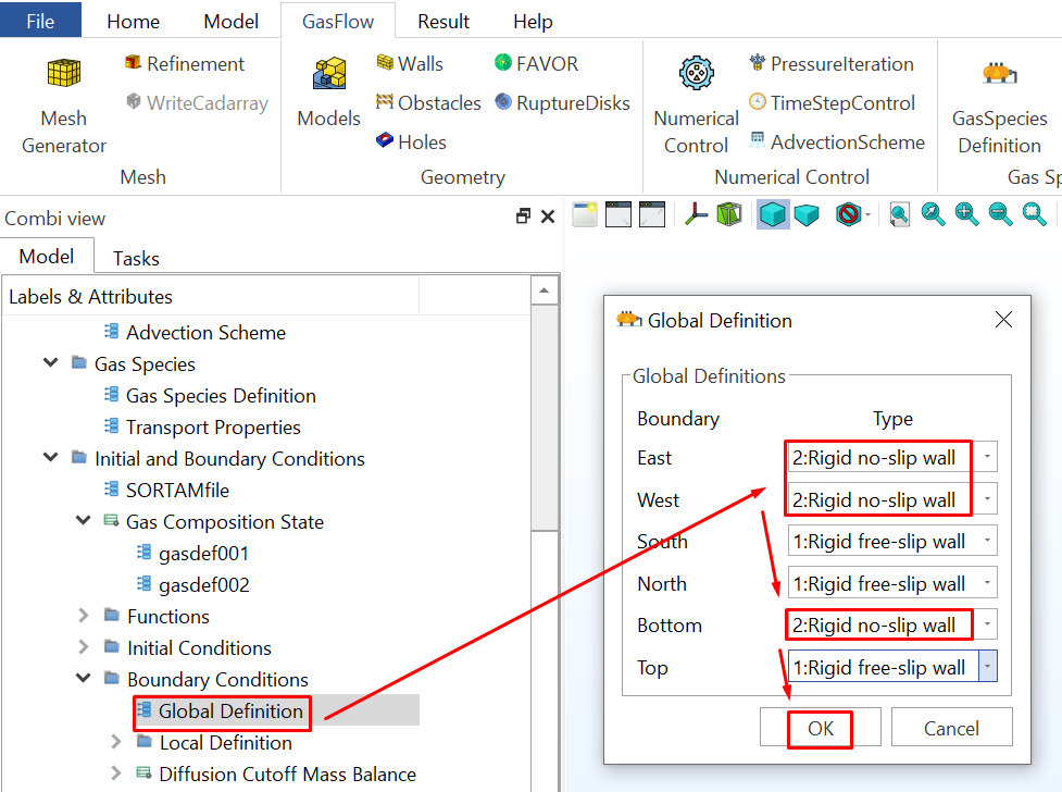
7.1 Set up the East/West and Bottom/Top boundaries as the rigid no-slip walls. The South/North boundaries are set as the rigid free-slip walls since there is only one cell in Y direction.
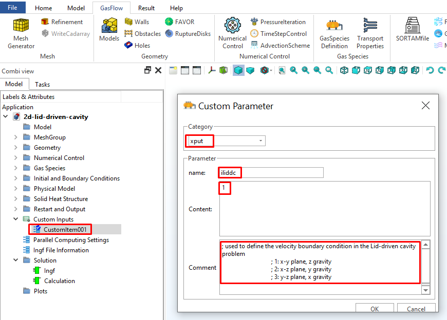
7.2 Activate the special velocity boundary condition developed for the 2-D Lid-driven cavity problem by inputting "iliddc" in the "Custom Parameter". It is especially useful for the input parameters that is unavailable in GASVIEW.
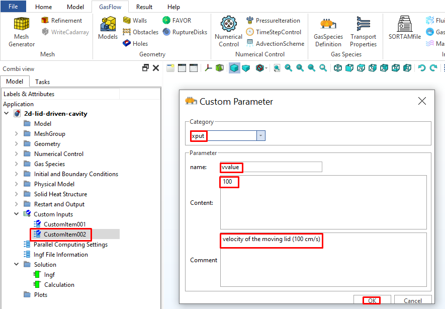
7.3 Set the velocity of the moving lid at 100 cm/s by adding "vvalue" in the "Custom Parameter".
Step 8. Physical Models
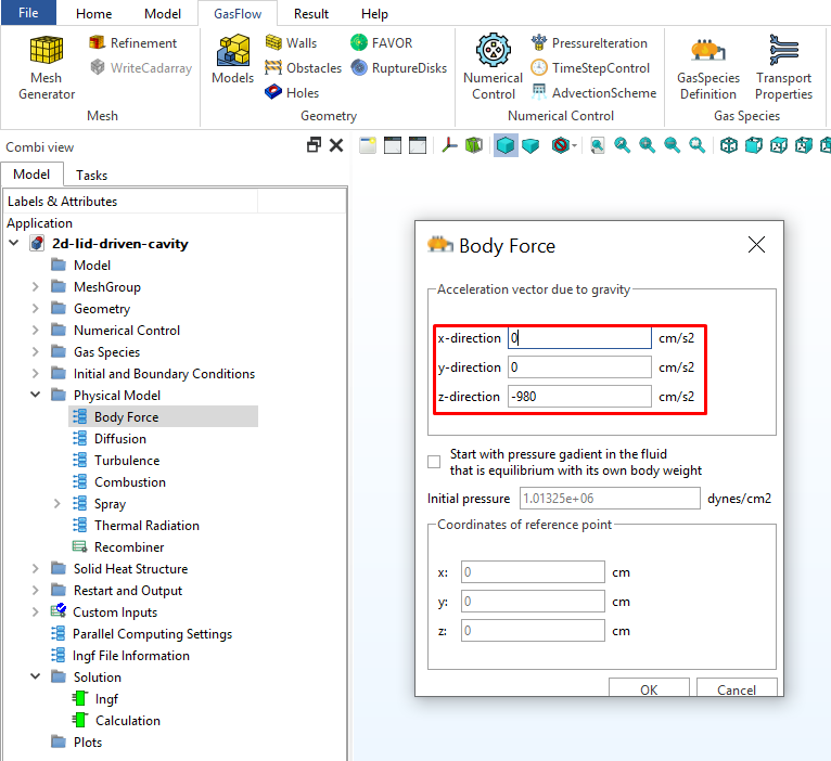
8.1 Set up the gravitational force.
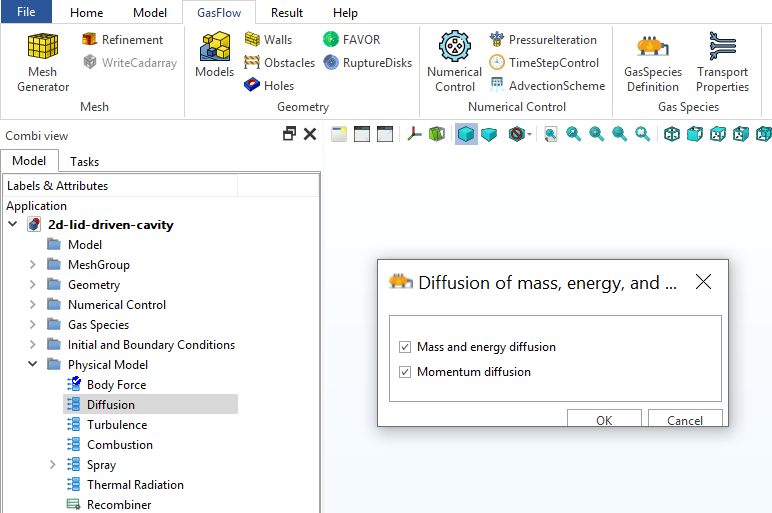
8.2 Set up the options for mass, momentum and energy diffusions.
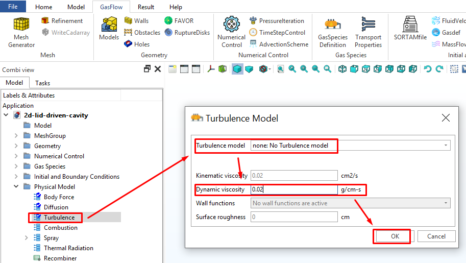
8.3 Set the turbulence model as "none". No turbulence model is required in this Lid-driven cavity problem since the flow is laminar.
Step 9. Restart and Outputs
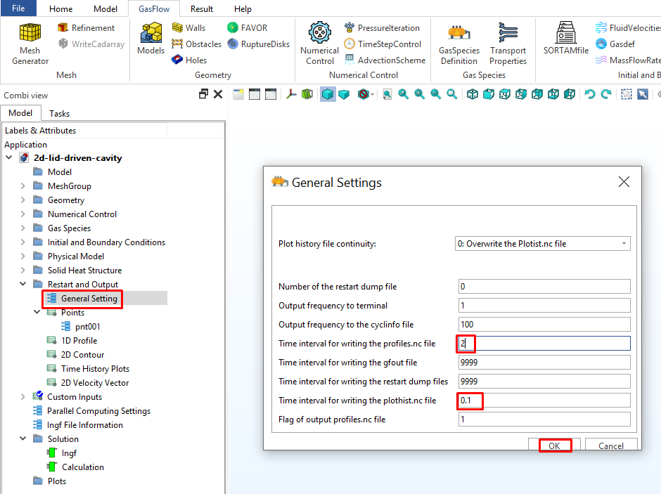
9.1 General options. Set the time intervals for writing the profiles.nc and plothist.nc to 2 s and 0.1, respectively.
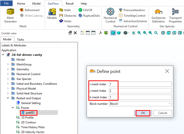
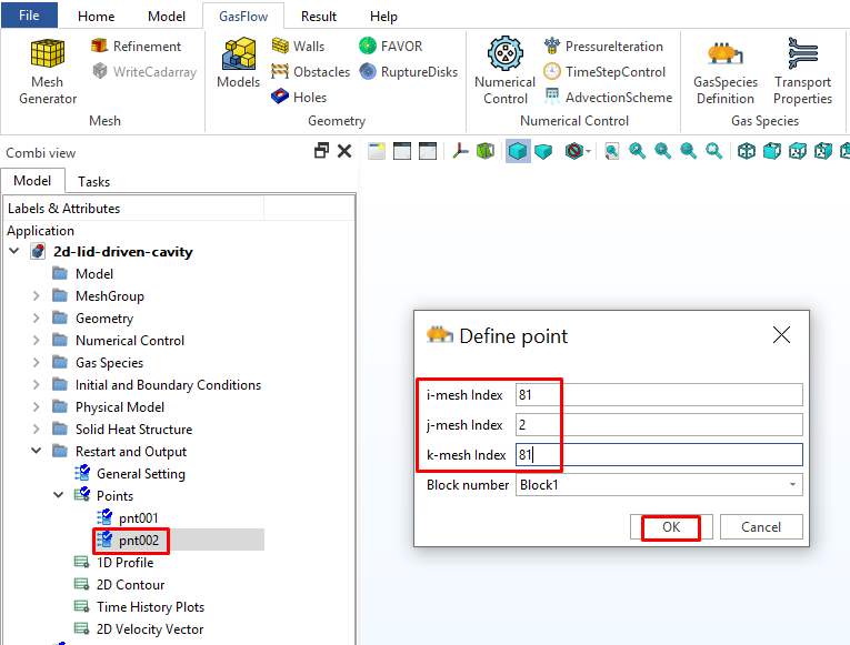
9.2 Set two points: pnt001 (i=1, j=2, k=1) and pnt002 (i=81, j=2, k=81) used to define a 2D plane.
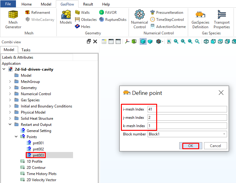
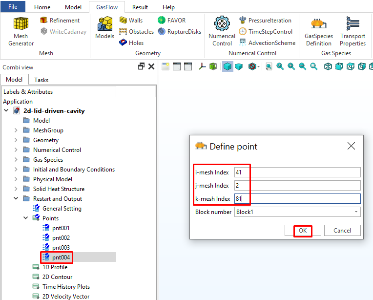
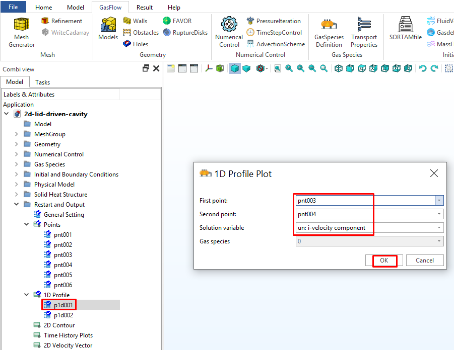
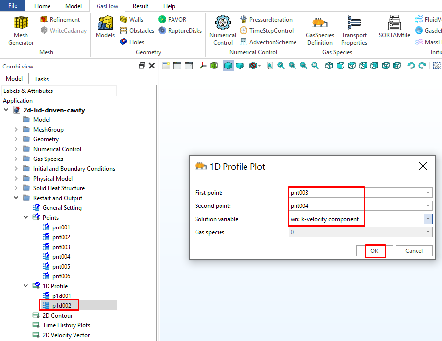
9.3 Set two points: pnt003 (i=41, j=2, k=1) and pnt004 (i=41, j=2, k=81) used to define the vertical centerline.
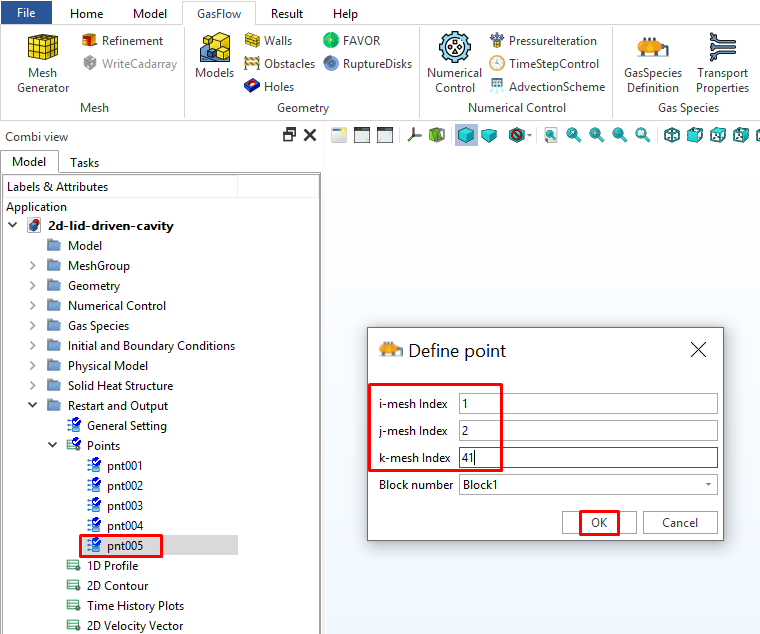
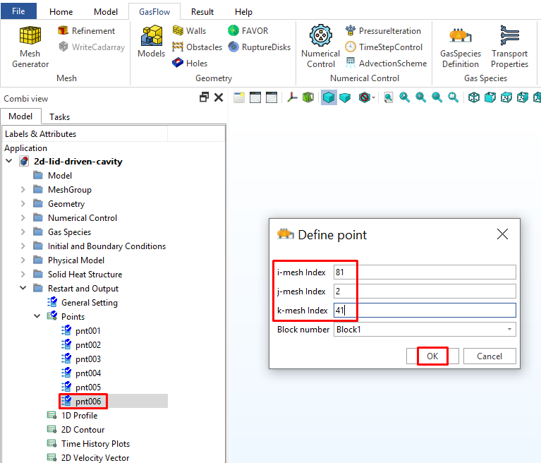
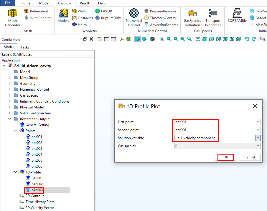
9.4 Set two points: pnt005 (i=1, j=2, k=41) and pnt006 (i=81, j=2, k=41) used to define the horizontal centerline.
9.5 Define 1D profiles along the centerlines to plot the variables "i-velocity component" and "k-velocity component".

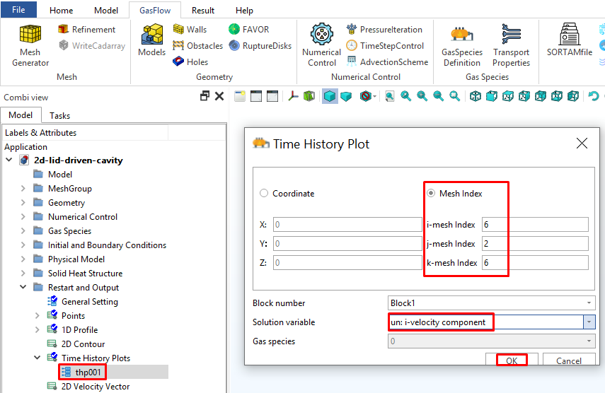
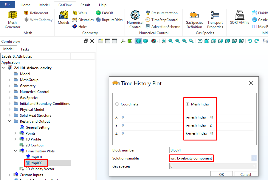
9.6 Define a monitor point at the corner (i = 6, j = 2, k = 6) and a monitor point at the center (i = 41, j = 2, k = 41) to plot the time histories of velocities. They are used to show if the steady state has been reached.
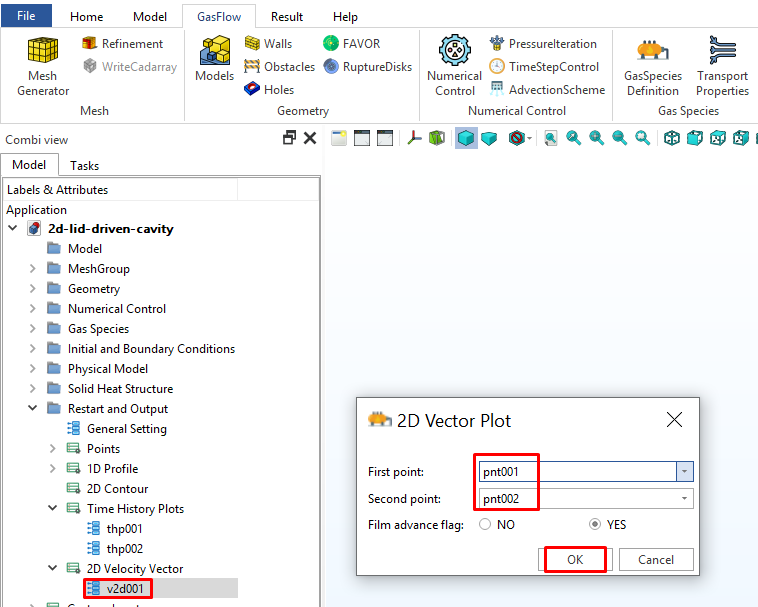
9.7 Use pnt001 and pnt002 to define a 2D plane v2d001 to plot the velocity vectors.
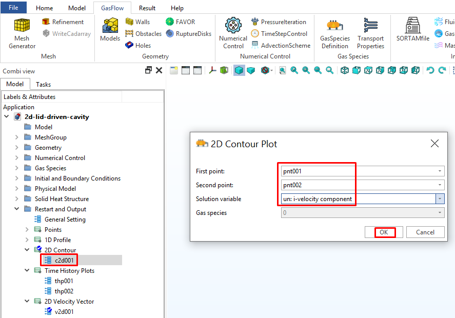
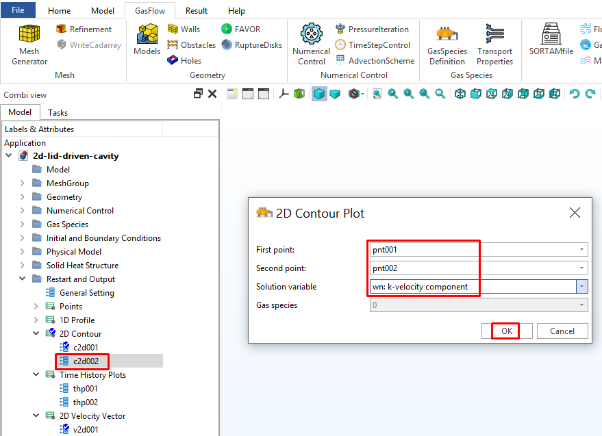
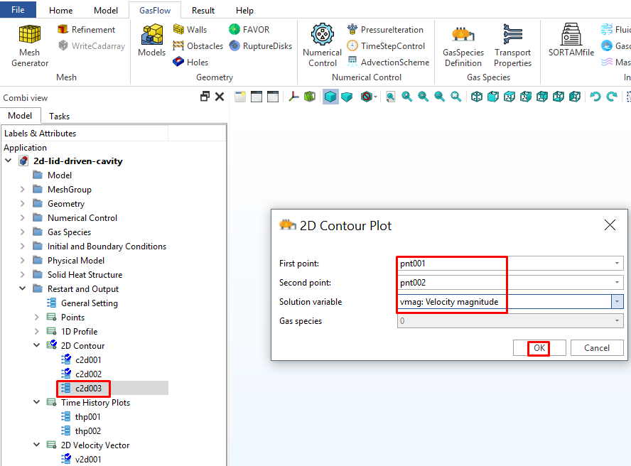
9.8 Use pnt001 and pnt002 to define 2D planes c2d001, c2d002 and c2d003 to plot the i-velocity "un", k-velocity "wn" and velocity magnitude "vmag".
Step 10. Generate Input File
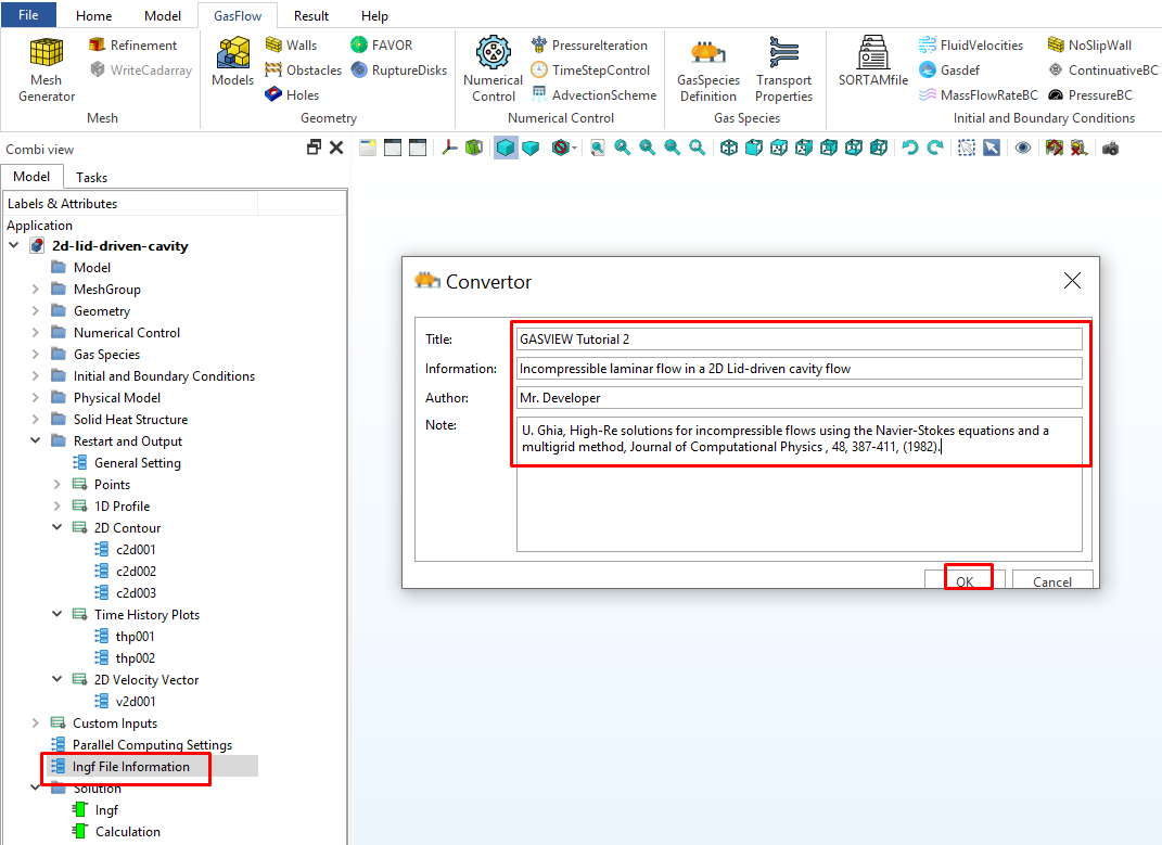
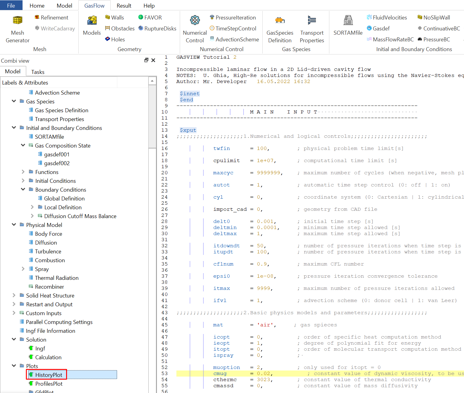
10.1 Click "Ingf File Information". Input the information and click "OK" to automatically generate the input file.
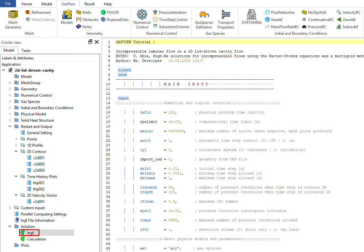
10.2 Click "Ingf" to review the input file.
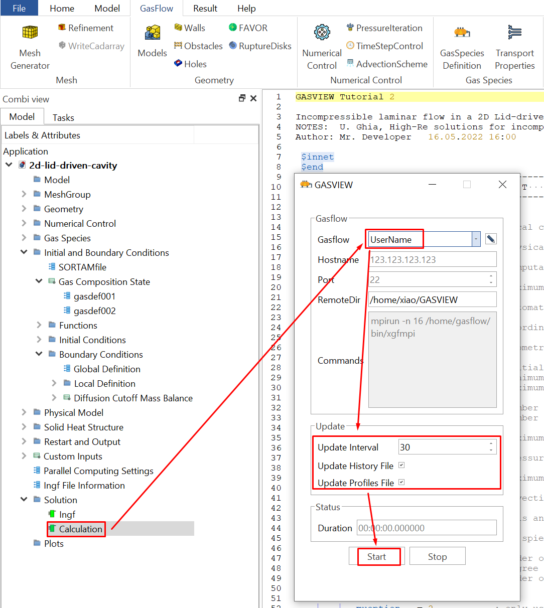
Step 11. Run Simulation
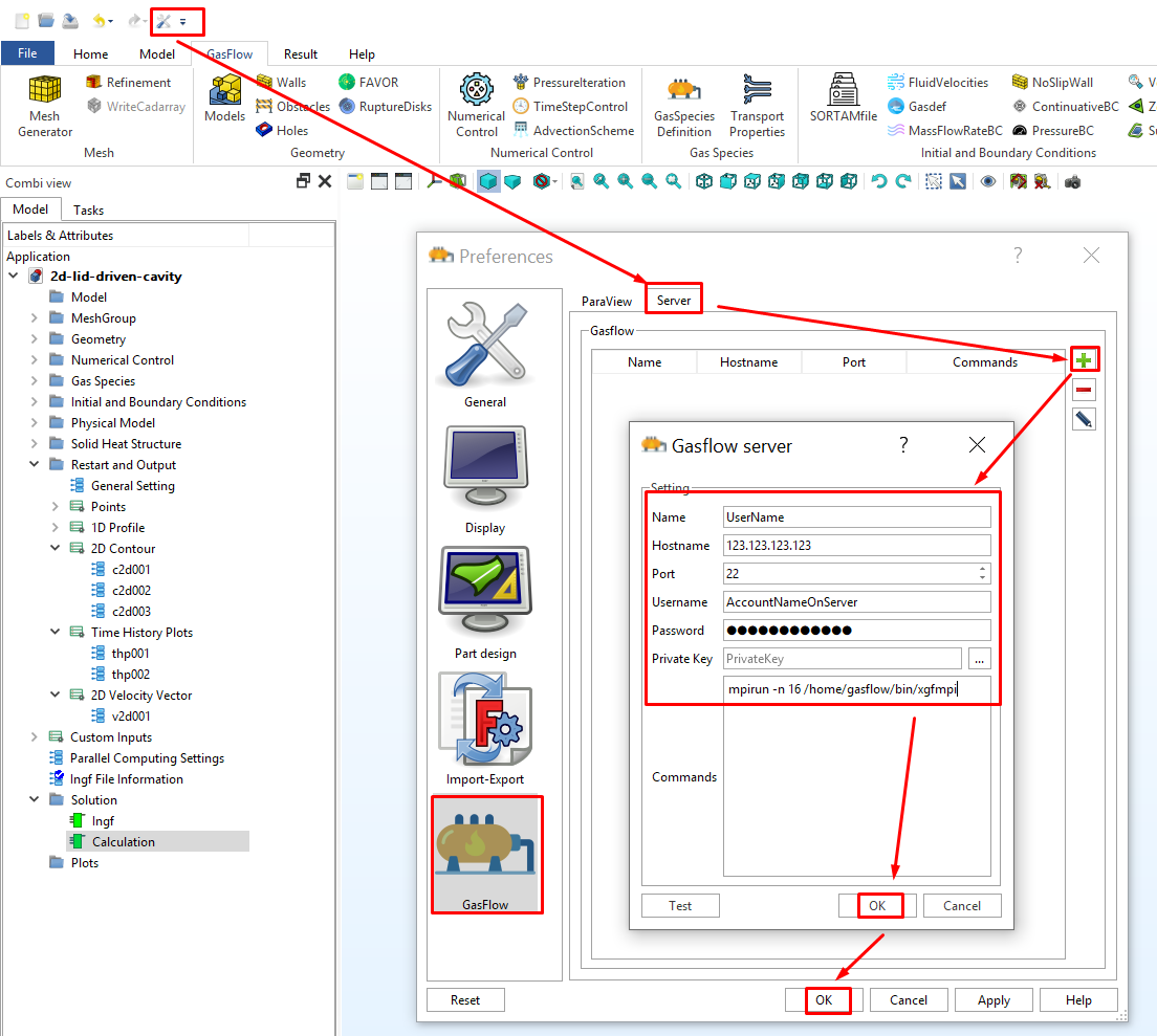
11.1 Set up the GASFLOW server. The user has to consult the server administrator regarding the account information.
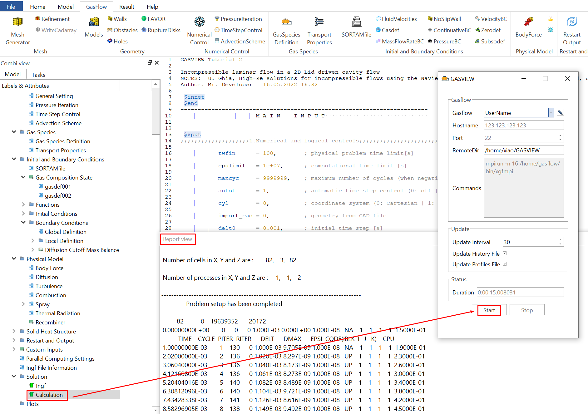
11.2 Click "Calculation", input the running directory and start to run GASFLOW.
11.3 The calculation cycle information is shown in the "Report View".
Step 12. Post-processing with GASVIEW
In this tutorial, we will show how to visualize the results using the tool in the GASVIEW. It provides a fast way to check the GASFLOW results during the calculation. After the calculation is finished, the user can use the more powerful pyscan and ParaView for visualization purposes.
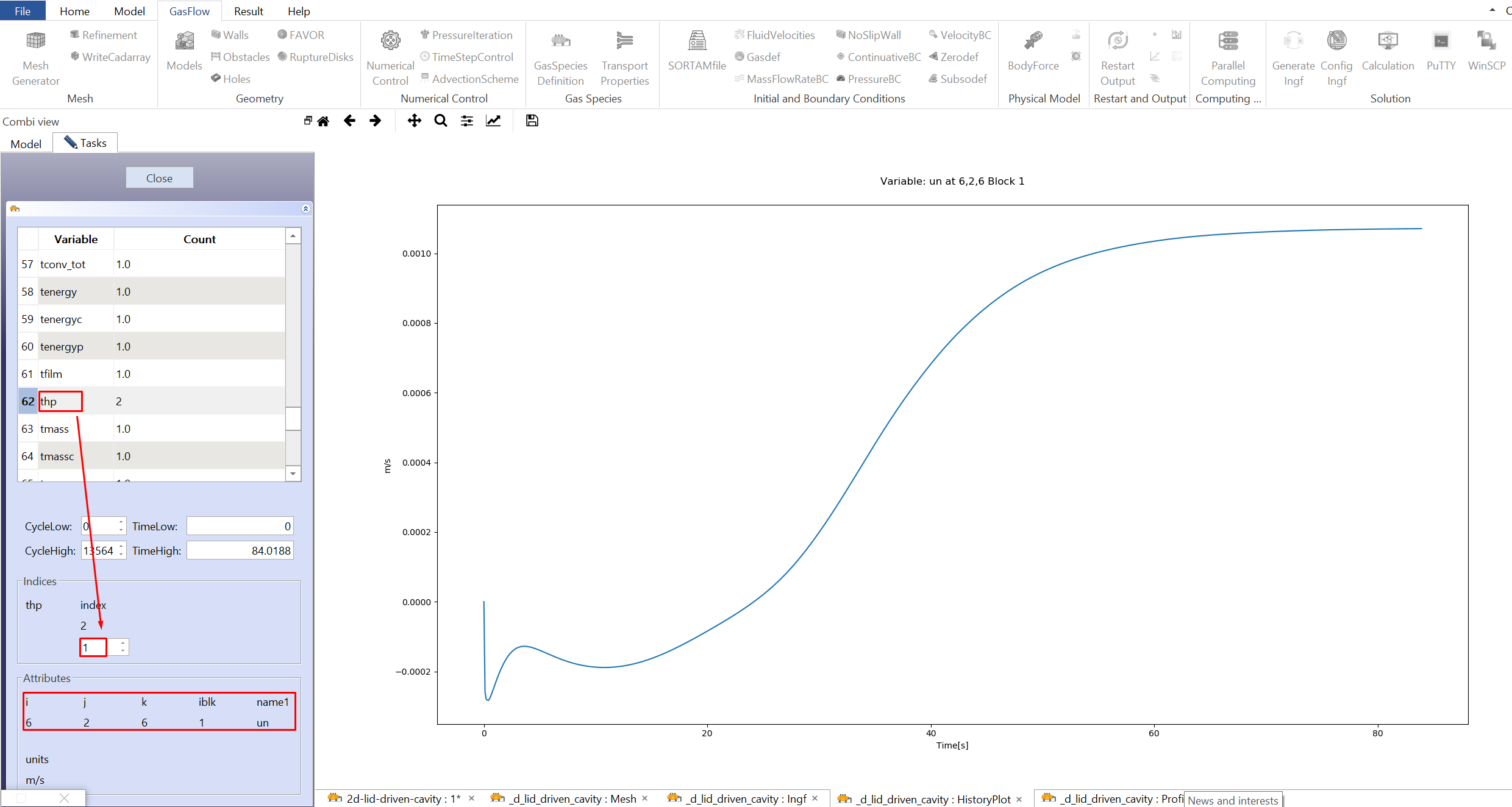
12.1 Click "Plots" - "HistoryPlot" to draw the time history plots.
12.2 Click "thp" to plot time history of the variables defined in Step 9.
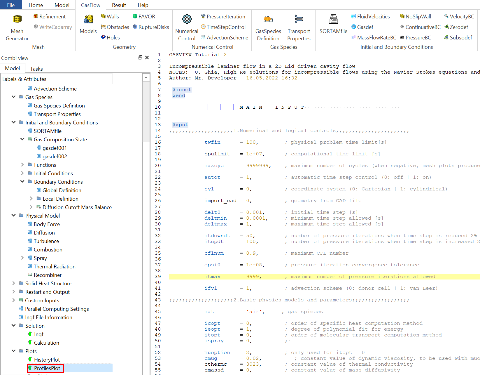
12.3 Click "ProfilesPlot" to plot 1D profiles of the variables defined in Step 9.
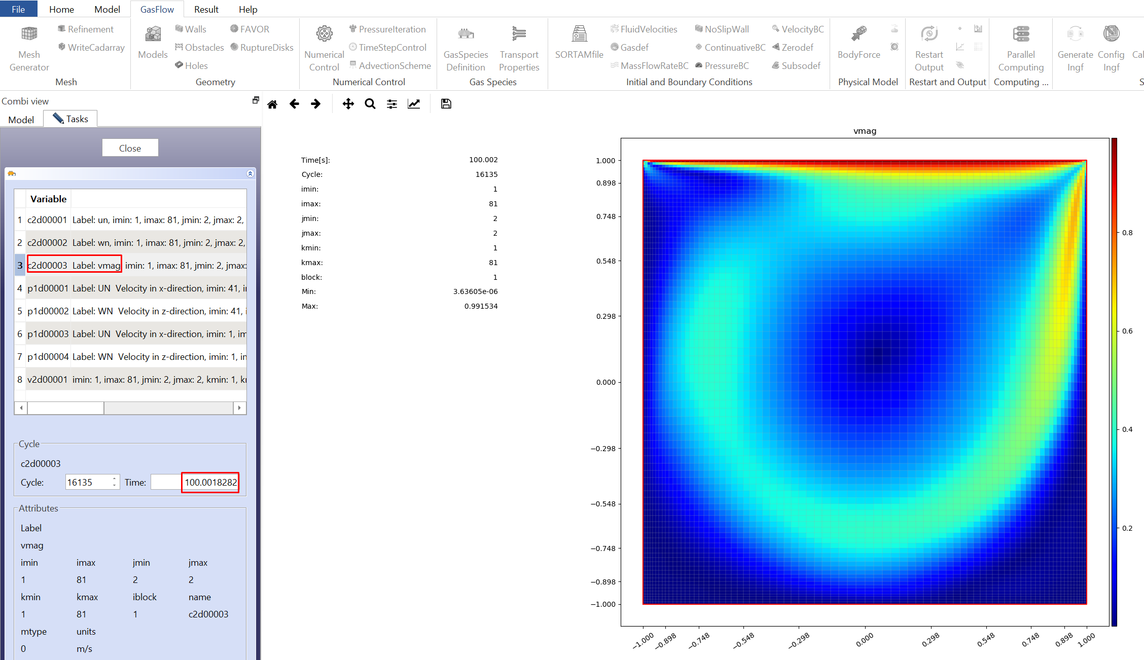
12.4 Select "c2d00003" to plot 2D cut of the velocity magnitude. The picture below shows the velocity magnitude at 100 s.
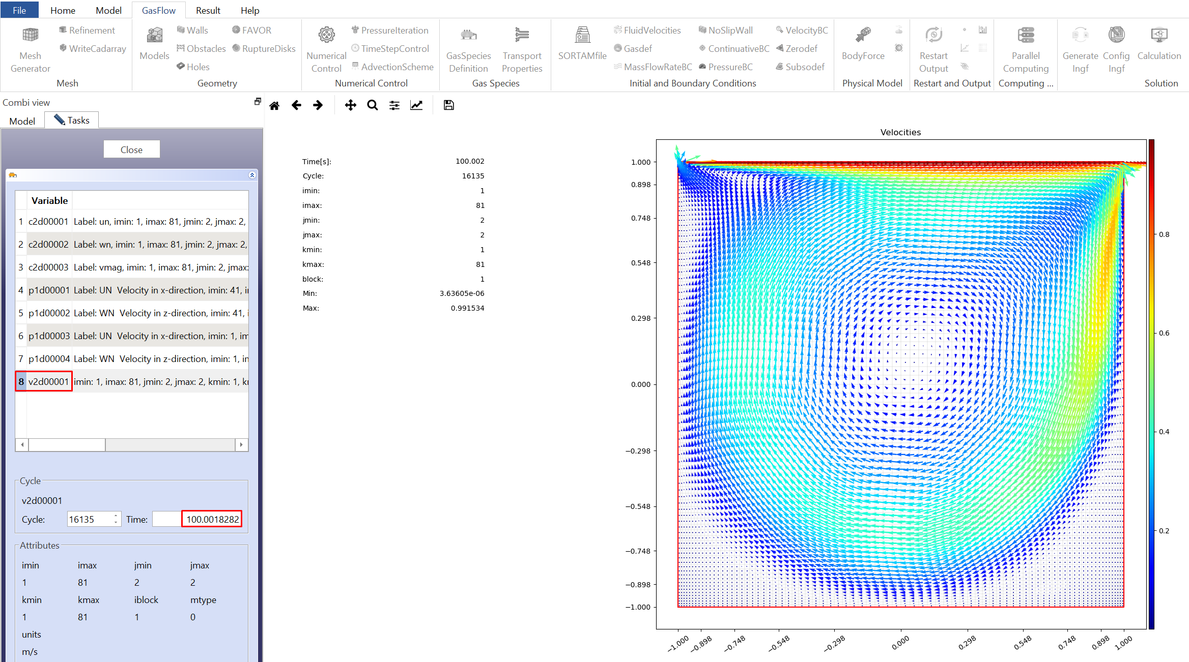
12.5 Select "v2d00001" to plot 2D cut of the velocity vectors. The picture below shows the velocity vectors at 100 s.
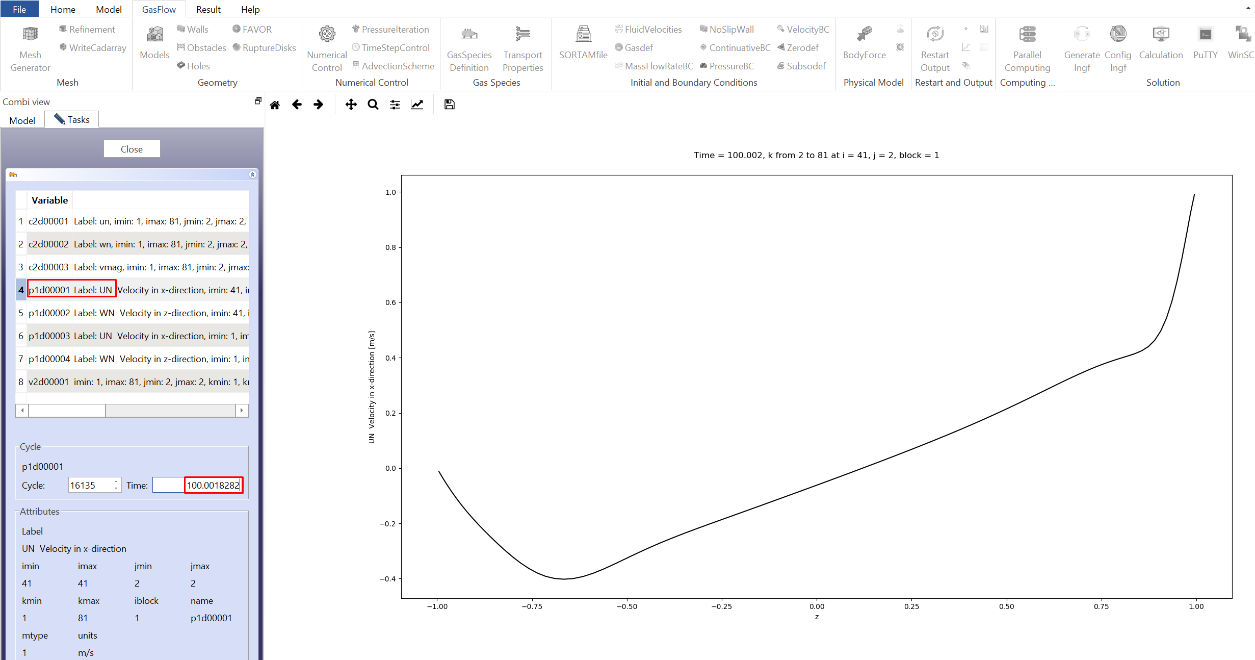
12.6 Select "p1d00001" to plot 1D profile of the x-velocity component along the vertical centerline. The picture below shows the x-velocity at 100 s.
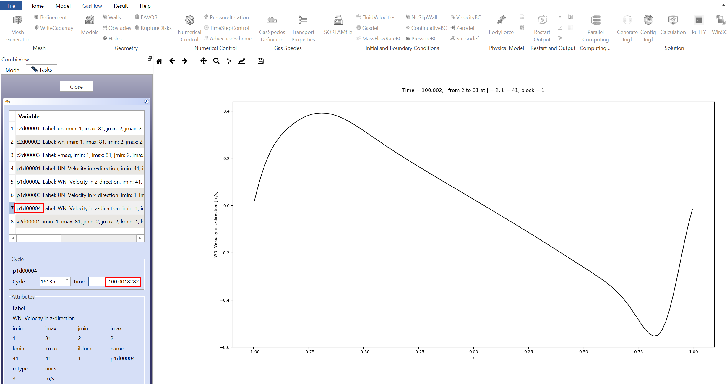
12.7 Select "p1d00001" to plot 1D profile of the z-velocity component along the horizontal centerline. The picture below shows the z-velocity at 100 s.